Let M = (Q, Σ, δ q0, F) be a DFA. The transition function δ : Q × Σ → Q, when interpreted in terms of the DFA's state graph, says that δ(q,a) = s corresponds to there being a transition labeled a going from state q to state s. We define the extended version of δ, called δ*, as follows:
| δ*(q,λ) | = | q |
| δ*(q,xa) | = | δ(δ*(q,x),a) |
From the definition you can infer that its signature is δ* : Q × Σ* → Q. In terms of the state graph of M, δ*(q,x) = s corresponds to the statement that the walk labeled x beginning in state q ends in state s. (The label of a walk is the concatenation of the labels on the transitions along the walk.)
Here we are interested in taking a DFA M and minimizing it, which is to say producing the smallest DFA M' such that L(M) = L(M'). It turns out that this task boils down to partitioning the states of M in accord with the indistinguishability relation on states and then merging every equivalence class into a single state.
Two states s and q in M are said to be indistinguishable if, for every string x ∈ Σ*, δ*(s,x) and δ*(q,x) are either both accepting states or both non-accepting states.
Clearly, indistinguishability is an equivalence relation1. Let's call it I. For p ∈ Q, let [p] be the equivalence class of I containing state p. It can be shown that M recognizes the same language as M' = (Q',Σ,δ',[q0], F'), where Q' = {[q] | q ∈ Q}, F' = { [s] | s ∈ F }, and δ'([q],a) = [s] iff [δ(q,a)] = [s].
That δ' is well-defined depends upon the fact that if [s] = [q], then [δ(s,a)] = [δ(q,a)] for all a ∈ Σ.
This construction of M' from M simply takes each equivalence class of I and collapses all of its members into a single state. The result is that no two states of M' are indistinguishable and, moreover, L(M) = L(M'). Hence, M' is a minimal DFA recognizing L(M). It turns out that any two minimal DFAs recognizing the same language are isomorphic to each other, which is to say that they are essentially duplicates of one another. (A proof of this is outside the scope of this document.)
This raises the question of how to compute I. One standard approach is to successively compute I0, I1, I2, ..., (each of which is a subset of its predecessor) which eventually converges to I. Intuitively, (r,s) ∈ Ik (k≥0) iff states r and s are indistinguishable by every string of length k or less, by which is meant that, for all x ∈ Σ≤k, δ*(r,x) and δ*(s,x) are either both accepting or both non-accepting.
Each Ik+1 is a refinement of Ik, meaning that the former is a subset of the latter or, equivalently, each equivalence class in the latter is the union of equivalence classes (possibly only one!) of the former. Yet another way to say it is that each equivalence class of Ik+1 is a subset of some equivalence class of Ik.
Note that if Ik+1 = Ik, then Ij = Ik for all j≥k. If the DFA in question has n states, this means that I = In−1.
What makes it convenient to compute the Ik's is the following:
Theorem:
| (r,s) ∈ I0 | ≡ | (r ∈ F) = (s ∈ F) |
| (r,s) ∈ Ik+1 | ≡ | (r,s) ∈ Ik ∧ (δ(r,a), δ(s,a)) ∈ Ik for all a ∈ Σ |
This says that (r,s) ∈ I0 (in words, states r and s are 0-indistinguishable) iff either they are both accepting or both nonaccepting. Meanwhile, (r,s) ∈ Ik+1 (r and s are (k+1)-indistinguishable) iff r and s are k-indistinguishable and, for each letter of the input alphabet, the transitions from r and s on that letter go to states that are k-indistinguishable from each other.
Assume that M = (Q,Σ,δ,q0,F), where Q = { qi | 0≤i<n }.
Among the variables employed in this algorithm are:
Within the comments of the algorithm, IN_DIST refers to the relation described by the current value of inDist[][]. That is, IN_DIST = { (p,q) | inDist[p][q] }.
The algorithm operates by repeatedly discovering "new" pairs of states that are distinguishable from each other, until such time as no such pairs exist. At that point, IN_DIST = I, which is to say that the relation described by inDist[][] is precisely I, meaning that it correctly indicates, for each pair of states, whether or not they are indistinguishable.
Because indistinguisability is a symmetric relation, we need to use only half of the elements of inDist[][]. Specifically, only elements inDist[k][j], where 0≤j≤k<n, are needed. (These are the elements on the main diagonal or above. We could have chosen to use the elements on the main diagonal or below.) For this reason, in practice we would make inDist an array of arrays of type boolean[] in which, for each k satisfying 0≤k<n, inDist[k] would be an array of length k+1. (Arrays whose elements are arrays, possibly of different lengths, are sometimes called "ragged" arrays.)
// Matrix representing partially computed I.
// Let IN_DIST = { (p,q) | inDist[p][q] }
boolean[0..n)[0..n) inDist;

// Initialize inDist[][] so that IN_DIST = I0
do for i in [0..n)
|  inDist[i][i] := true
|  do for j in [0..i)
|  |  inDist[i][j] := (qi ∈ F) ≡ (qj ∈ F)
|  od
od

int r := 0     // for counting iterations of outermost loop
boolean changed := true  // did IN_DIST change during current iteration?
// loop invariant: I ⊆ IN_DIST ⊆ Ir
do while changed
|  changed := false
|  // loop invariant: I ⊆ IN_DIST ⊆ Ir
|  do for i ∈ [1..n)
|  |  // loop invariant: I ⊆ IN_DIST ⊆ Ir
|  |  do for j ∈ [0..i)
|  |  |  if inDist[i][j] then
|  |  |  |  // loop invariant: I ⊆ IN_DIST ⊆ Ir
|  |  |  |  do for a ∈ Σ
|  |  |  |  |  k := δ(qi,a)
|  |  |  |  |  m := δ(qj,a)
|  |  |  |  |  if ¬inDist[k max m][k min m] then
|  |  |  |  |  |  inDist[i][j] := false
|  |  |  |  |  |  changed := true
|  |  |  |  |  fi
|  |  |  |  od
|  |  |  fi
|  |  od
|  od
|  r := r+1
od
|
We now analyze the algorithm, which is essentially a loop followed by another loop. The first loop, which iterates with i going through the range 0..n-1, has nested within it a loop that iterates with j going through the range 0..i-1. This pattern should be familiar to you by now. It results in the nested loop iterating a total of 0+1+2+...+(n−1) times, which comes out to (n2−n)/2 iterations. Each iteration of the nested loop takes constant time, which means that this portion of the program completes in O(n2) time. Now consider the second loop, which we refer to as the changed-loop, as the variable of that name determines when it terminates. It has nested within it a loop having control variable i; within that loop is a loop having control variable j. (Call these the i-loop and j-loop.) The i-loop iterates with i going from 1 through n−1. Meanwhile, the j-loop iterates with j going from 0 through i-1, which is i iterations. This is essentially the same pattern as we saw above, and it results in the j-loop iterating 1+2+3+...+(n−1) times, or (n2−n)/2 times, during each iteration of the changed-loop.
If we consider |Σ| to be a constant, which is the convention, we get that each iteration of the j-loop takes constant time. Which means that each iteration of the changed-loop takes O(n2) time. But how many times does the changed-loop iterate? In the worst case, n times.2
Which means that the changed-loop runs in time O(n3). As that loop's running time exceeds the first one's we get that the algorithm's asymptotic running time corresponds to that of the changed-loop, O(n3).
The naive algorithm above has a "brute-force" feel to it in the sense that, when it finds a pair of states to be distinguishable, there is no effect upon "where it looks next" to find more such pairs of states. A somewhat more sophisticated algorithm would, when a pair of states (p,s) is found to be distinguishable, turn its attention to pairs of states that are distinguishable as a consequence of (p,s) being so.
The algorithm presented below does what is suggested above. Specifically, each time a pair of states (p,s) is found to be distinguishable, it is placed onto a queue. When it reaches the front of the queue (and is removed therefrom), any pair of states (k,m) whose indistinguishability depends upon p and s being indistinguishable will be recognized as being distinguishable! If, for some a ∈ Σ, δ(k,a) = p and δ(m,a) = s, then (k,m) is such a pair of states. Which is to say that the set of pairs of states whose indistinguishability depends upon that of p and s is the union, over all a ∈ Σ, of δ-1(p,a) × δ-1(s,a). (By δ-1(p,a) is meant the set of states whose outgoing transition on a goes to state p. In other words: {r : δ(r,a) = p}.)
 (1) boolean[0..n)[0..n) inDist  // represents partially computed I
 (2) Queue<int,int> q

     // Initialize inDist so that inDist[i][j] iff (qi, qj) ∈ I0
     // and the queue to contain all pairs of states that are not in I0
 (3) q := emptyQueue;
 (4) do for i in [0..n)
 (5) |  inDist[i][i] := true;
 (6) |  do for j in [0..i)
 (7) |  |   if (qi ∈ F) ≡ (qj ∈ F) then
 (8) |  |   |  inDist[i][j] := true
 (9) |  |   else
(10) |  |   |  inDist[i][j] := false
(11) |  |   |  q.enqueue(<i,j>)
(12) |  |   fi
(13) |  od
(14) od

(15) do while !q.isEmpty()
(16) |  <i,j> := q.front()   // i and j are distinguishable
(17) |  q.dequeue()
(18) |  do for a ∈ Σ
(19) |  |  SetOfInt A := δ-1(i,a)
(20) |  |  SetOfInt B := δ-1(j,a)
     |  |  // each pair in A×B is distinguishable
(21) |  |  do for each (k,m) ∈ A×B
(22) |  |  |  k', m' := k max m, k min m;  // simultaneous assignment
(23) |  |  |  if inDist[k'][m'] then
(24) |  |  |  |  inDist[k'][m'] := false;
(25) |  |  |  |  q.enqueue(<k', m'>)
(26) |  |  |  fi
(27) |  |  od
(28) |  od
(29) od
|
This improved algorithm is more difficult to analyze than was the naive algorithm shown earlier. Like the naive algorithm, this one is composed of two loops. We refer to them, respectively, as the initialization-loop and the main-loop. As in the naive algorithm, it is obvious that the initialization-loop takes O(n2) time.
The main-loop has two loops nested inside it. Because, by convention, we assume that the input alphabet Σ is constant in size, we can treat the loop that iterates once for each member of Σ as though it iterates only once, for some arbitrary member a of Σ. In other words, we can pretend that Σ has only one member.
The key to showing that the improved algorithm's running time is O(n2) is demonstrating that the most deeply nested loop within the main-loop iterates only that many times, taken over all iterations of the main-loop. This reduces to showing that, taken over all iterations of the main-loop, the sum of the sizes of the sets A×B is O(n2). Toward that end, we state the following two lemmas.
Lemma 1: Let i and i' be distinct states. Then
δ-1(i,a) ∩ δ-1(i',a) = ∅
Proof: Suppose otherwise, and let k be a member of both
δ-1(i,a) and δ-1(i',a).
But then δ(k,a) = i ≠ i' = δ(k,a), which implies,
contrary to what we know, that δ is not a function.
■
Lemma 2: Let [i,j] and [i',j'] be distinct pairs of states,
and let A = δ-1(i,a), A' = δ-1(i',a),
B = δ-1(j,a), and B' = δ-1(j',a).
Then A×B ∩ A'×B' = ∅
Proof: Because [i,j] and [i',j'] are distinct pairs, either
i≠i' or j≠j'. Without loss of generality, assume the former.
By Lemma 1, A ∩ A' = ∅, which implies the result.
■
Consider two distinct iterations of the main loop, where the pair of states [i,j] is taken from the front of the queue in one iteration and [i',j'] in the other. Examination of the algorithm, in particular lines 23-26, make it clear that no ordered pair of states is placed on the queue more than one time. Thus, [i,j] and [i',j'] are distinct pairs. Let A, A', B, and B be as described in the statement of Lemma 2. Then Lemma 2 tells us that A×B ∩ A'×B' is empty, which is to say that on no two iterations of the main loop will the same pair (k,m) be considered in the loop of lines 21-27. That is, taken over all iterations of the main loop, the loop of lines 21-27 will iterate at most once for each pair of states. In fact, it will iterate once for each pair of states that is distinguishable. As the number of such pairs is at most n(n−1)/2, we have the desired result.
| δ | inputs | |
|---|---|---|
| state | a | b |
| 1 | 3 | 7 |
| 2 | 6 | 8 |
| 3 | 2 | 1 |
| 4 | 5 | 7 |
| 5 | 2 | 4 |
| 6 | 7 | 9 |
| 7 | 3 | 4 |
| 8 | 4 | 4 |
| 9 | 1 | 8 |
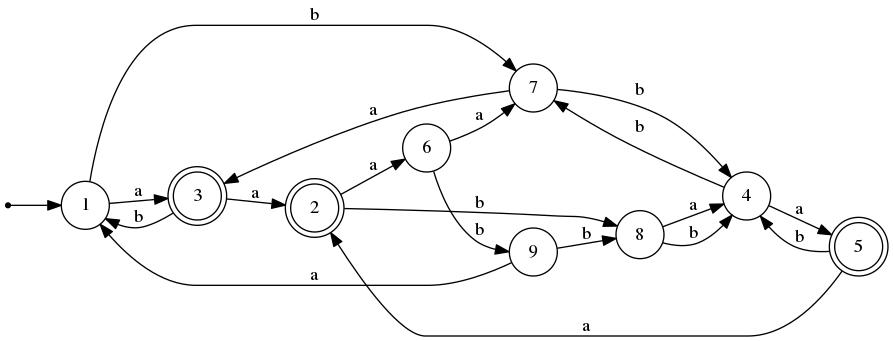
We describe the algorithm by means of an example, applying it to the DFA M = (Q, Σ, δ, q0, F), where Q = {1,2,...,9}, {a,b}, Σ = {a,b}, q0 is state 1, F = {2,3,5}, and δ is as described in the table to the right.
The algorithm begins, not unlike the ones described earlier, by constructing a representation of I0. The algorithm is iterative, with the k-th iteration of the loop beginning with a representation of Ik−1 and finishing by having produced a representation of Ik. For some k, it will be that Ik-1 and Ik are identical. At that point the algorithm terminates, as I = Ik−1 and the equivalence classes of I will have been determined.
In contrast to the algorithms described earlier, this one's representation of the partially computed version of equivalence relation I (i.e., Ik for some k) is not in the form of a boolean matrix but rather as a set of sets, or a set of lists, where each list contains the members of one equivalence class.
For purposes of referring to the equivalence classes, we choose one member from each class —by convention, the lowest-numbered state— and make it the representative of that class. If, for example, state 5 were the representative of its class, we would refer to the class by [5] (the state ID enclosed in square brackets).
During each iteration of the loop, for every equivalence class containing more than one member, we compute the "signature" of each of its members, which identifies the equivalence classes of the states to which its outgoing transitions go. Any two members of an equivalence class having distinct signatures are thereby discovered to be distinguishable and thus will appear in distinct equivalance classes during the next iteration of the loop. (This is to say that the two states in question are (k−1)-indistinguishable but not k-indistinguishable.)
I0 has two equivalence classes: the accepting states form one and the non-accepting states form the other. That is where we begin. The following depicts what happens during the first iteration of the algorithm as applied to the example DFA.
             Round 1
      [2]                  [1]
  -----------    -----------------------
   2   3   5      1   4   6   7   8   9
a [1] [2] [2]    [2] [2] [1] [2] [1] [1]
b [1] [1] [1]    [1] [1] [1] [1] [1] [1]
|
The equivalence classes of I0 are [2] = {2,3,5} (the accepting states) and [1] = {1,4,6,7,8,9} (the non-accepting states). The column under each state ID is its computed signature. For example, state 5's signature is ⟨a→[2], b→[1]⟩ because δ(5,a) = 2, and 2 is a member of equivalence class [2] and δ(5,b) = 4, and 4 is a member of equivalence class [1].
Due to the fact that states 2 and 3 have distinct signatures, we determine that, while they are 0-indistinguishable (i.e., (2,3) ∈ I0), they are not 1-indistinguishable (i.e., (2,3) ∉ I1). On the other hand, states 3 and 5 have the same signature, so they are not only 0-indistinguishable but also 1-indistinguishable.
The states in equivalence class [1] have two distinct signatures, so, like equivalence class [2], they must be split into two classes.
Having split each equivalence class into two of them, Round 2 looks like this:
                 Round 2

   [2]     [3]         [1]           [6]
   ---   -------   -----------   -----------
    2     3   5     1   4   7     6   8   9
a   -    [2] [2]   [3] [3] [3]   [1] [1] [1]
b   -    [1] [1]   [1] [1] [1]   [6] [1] [6]
|
Because state 2 is alone in its equivalence class, and thus class [2] cannot be split, there is no need to compute its signature. We see that the states in [3] have the same signatures, as do those in [1]. Thus, those two equivalence classes advance, intact, to the next round. However, the signatures of the states in [6] indicate that state 8 is distinguishable from states 6 and 9. So we must carry out another round:
                 Round 3

   [2]     [3]         [1]         [6]     [8]
   ---   -------   -----------   -------   ---
    2     3   5     1   4   7     6   9     8
a   *    [2] [2]   [3] [3] [3]   [1] [1]    *
b   *    [1] [1]   [1] [1] [1]   [6] [8]    *
|
This round finds that states 6 and 9 are distinguishable. So we split up [6] into two equivalence classes and do yet another round:
                 Round 4

   [2]     [3]         [1]       [6]   [8]   [9]
   ---   -------   -----------   ---   ---   ---
    2     3   5     1   4   7     6     8     9
a   *    [2] [2]   [3] [3] [3]    *     *     *
b   *    [1] [1]   [1] [1] [1]    *     *     *
|
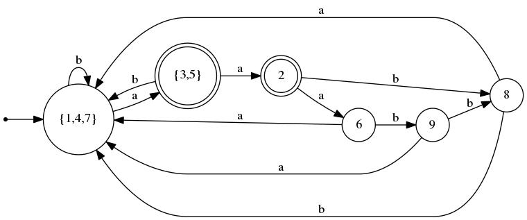
Within each equivalence class, the signatures of its states are identical. This being the 4th round, it means that we have determined that I3 = I4 = I. To produce the minimal DFA equivalent to the the given one, we take each equivalence class and merge its states into a single state. In our example, it means that states 1, 4, and 7 become a single state, as do states 3 and 5. The figure below shows the original DFA M and its equivalent minimal DFA M'.
| M: | |
| M': | |
If R ⊆ A×A is an equivalence relation, it partitions the elements of A into mutually disjoint equivalence classes A1, A2, ..., Am satisfying the condition that each a ∈ A is related by R to every element in its own equivalence class but to no elements in any other equivalence class.
By convention, the notation [a] (where a ∈ A) denotes the equivalence class of which a is a member, i.e., { b ∈ A | (a,b) ∈ R}.